Using a Convolutional Neural Network to Read American Sign Language

USING A CONVOLUTIONAL NEURAL NETWORK TO READ AMERICAN SIGN LANGUAGE

I was a sophomore in college the first time I ever witnessed somebody using American Sign Language (ASL) to communicate. Although I have no goal to learn ASL, it has always fascinated me how hand and facial movements can be used to have entire conversations all without uttering a single word. It was this fascination (along with finding an ASL dataset) that compelled me to create a convolutional neural network to classify American Sign Language letters.

The dataset I’m using was found on kaggle.com and includes 27,455 training images and 7,172 testing images. Each image shows a hand gesture in ASL representing a single letter in the alphabet except for the letters J and Z. These two letters aren’t included in the dataset because motion is required to express them and this dataset only includes images. Using this data, we’re able to create a neural network that’s capable of reading in an image and producing a prediction as to what letter that image represents.

A convolutional neural network (CNN) is used to analyze visual imagery and will be the heart of our ASL image classifier. The CNN is going to be built using Keras, a high-level Python API for the TensorFlow library. Before building the CNN, let's load the data and see exactly what we’re working with.

The data comes in the form of an excel file so it will be loaded with pandas’ read_csv() function.

DATA_DIR = "C:/Users/Fade/Desktop/sign_mnist"
training_data = pd.read_csv(DATA_DIR + "/sign_mnist_train.csv")
testing_data = pd.read_csv(DATA_DIR + "/sign_mnist_test.csv")

The read_csv() function returns a DataFrame object so calling training_data.head() returns the first 5 rows of the training data.

training_data.head()

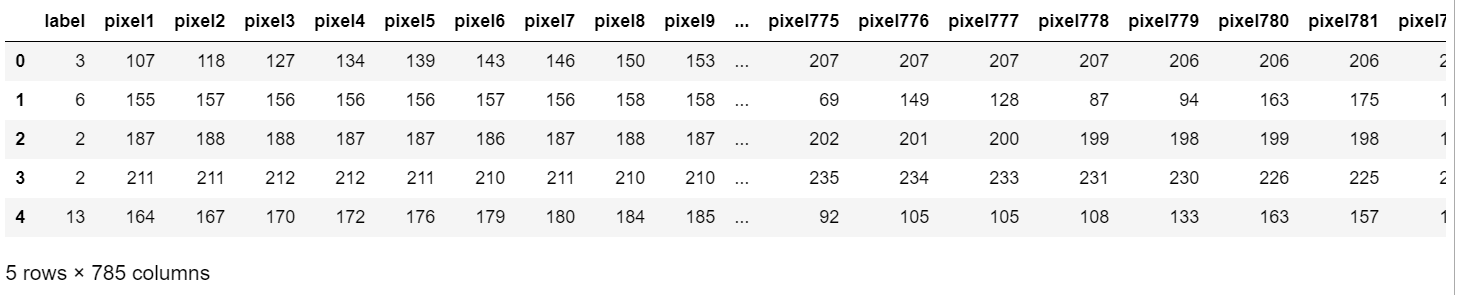
The first column ‘label’ represents a letter in the alphabet mapped numerically where A=0, B=1, C=2 and so on for all letters in the alphabet. Labels 9 and 25 aren’t included because they represent letters J and Z, respectively. Remember those two letters aren’t included in the dataset because they require motion to express them. Columns 2-784 represents a single 28x28 image where each value represents the grayscale value of the pixel. Grayscale values fall within the range of 0-255. When training and testing a CNN, images in the dataset should be resized to 28x28 because the CNN will perform a lot faster if all the images were scaled down. Having a bigger image only makes training and testing take longer and a large image isn’t required since the features in the image will still remain intact. Grayscale conversion is not required but since color is not a factor in this classification problem, it’s just unnecessary processing if we kept it. By converting it to grayscale, our CNN will take a shorter time to train and test. Normally, resizing the image and converting it to grayscale is something that we have to do ourselves. Thankfully, this dataset has already handled some of the data preprocessing.

When training and testing our CNN, it requires two things: The data itself and the label of each item in the data; both represented as a numpy array.

Loading the training and testing images:

X_train = training_data.drop(columns="label").to_numpy()
X_test = testing_data.drop(columns="label").to_numpy()

Loading the training and testing image labels:

y_train = training_data["label"].to_numpy()
y_test = testing_data["label"].to_numpy()

It’s great that we have our training and testing data and labels separated, but there is still a few more preprocessing we need to do on our data before building the CNN. Each pixel value in the training and testing data (X_train and X_test) have a value between 0-255. Our CNN will run much faster if we normalize the values to be between 0-1.

X_train = X_train/255
X_test = X_test/255

Below you can see the difference that it made. The following is the first 5 pixel values in the training data:

Before: [107 118 127 134 139]
After: [0.41960784 0.4627451  0.49803922 0.5254902  0.54509804]

Next we have to convert the numpy array of our training and testing data from a 1D shape (784 pixels) to a 3D shape (28, 28, 1). This is done because a 3D shape is required for the CNN to accept it as input:

X_train = X_train.reshape(-1, 28, 28, 1)
X_test = X_test.reshape(-1, 28, 28, 1)

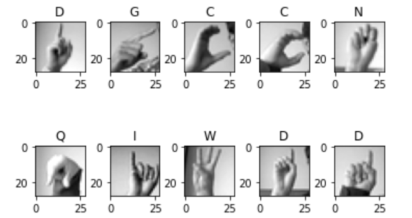
Now that we’re done with the data preprocessing for the images, let’s visualize them. Here are the first 10 images in the training set:

Finally, we need to transform the training and testing labels to be categorical. Thankfully, sklearn’s preprocessing module provides a class called LabelBinarizer which has a function called fit_transform() which converts a numpy array of integers into a matrix representation of each category. The CNN can’t be trained without performing this transformation.

label_binarizer = LabelBinarizer()
y_train = label_binarizer.fit_transform(y_train)
y_test = label_binarizer.fit_transform(y_test)

To better visualize this transformation, the first value of the training label is 3 (Letter D). After the transformation, the first value of the training label becomes a binary matrix, where all the positions in the matrix are 0 except for the 3rd index, which is 1.

Before: 3
After: [0 0 0 1 0 0 0 0 0 0 0 0 0 0 0 0 0 0 0 0 0 0 0 0]

If the label was 7 (Letter H), the transformation would look like this (notice the 7th index is a 1):

Before: 7
After: [0 0 0 0 0 0 0 1 0 0 0 0 0 0 0 0 0 0 0 0 0 0 0 0]

With all of our data ready, we can finally begin building our CNN. First we create a model variable and set it equal to a Sequential model. A sequential model allows us to build a neural network which has exactly one input tensor and one output tensor.

model = Sequential()

There’s a lot going on in this next snippet. First we add a Conv2D layer to the model. The Conv2D layer is the most important layer in our CNN. This is what makes our neural network a convolutional neural network. The Conv2D layer is responsible for detecting the different patterns or features in images. How does it detect features exactly? It all starts with the filter. In our Conv2D instantiation, we specified a filter size of (3, 3):

model.add(Conv2D(32, (3,3), activation='relu', padding='same', strides=1, input_shape=(28,28,1)))

This filter will convolve through our image and perform a convolutional operation on it. I’m not a mathematician, but the general idea is that it takes our image data (a numpy array) and “summarizes” it into a smaller numpy array. Performing this summarization takes our image data and generalizes it into features. For our case, our image starts out as a regular image of a hand representing some letter in the alphabet. The filter will then see this image and begin detecting different aspects of it such as edges, corners, circles, or general shapes. The more Conv2D layers the model has, the more filters are applied on it, which results in more sophisticated filters. What starts out as a simple edge detection filter may become a filter for detecting a fist, a finger, or a nail. With these filters, an assumption can be made on what letter that image represents. Here’s a visualization of a filter performing a convolutional operation on a matrix with a 3x3 filter:

Next, we add a MaxPool2D layer to our model:

model.add(MaxPool2D(pool_size=(2,2), padding='same', strides=2))

The MaxPool2D layer will reduce the dimensions of the output from the Conv2D layer. This is done by running a filter (in our case, we defined a pool_size of 2x2) and it will take the max value of each 2x2 area in the MaxConv2D input (Conv2D output). This reduces the number of pixels from the Conv2D output and in doing so reduces computational load and helps reduce overfitting of the model (more on overfitting later).

Finally, we add a Dropout layer and set the rate of dropout to 0.2 or 20%. This will randomly set 20% of the neurons to have a weight of 0 for one iteration. Doing so reduces overfitting.

model.add(Dropout(0.2))

Finally, we add the rest of our layers, compile the model, and return the model. Building of the neural network was wrapped in a function called build_nn():

def build_nn():
    model = Sequential()

    model.add(Conv2D(32, (3,3), activation='relu', padding='same', strides=1, input_shape=(28,28,1)))
    model.add(MaxPool2D(pool_size=(2,2), padding='same', strides=2))
    model.add(Dropout(0.2))

    model.add(Conv2D(64, (3,3), activation='relu', padding='same', strides=1))
    model.add(MaxPool2D(pool_size=(2,2), padding='same', strides=2))
    model.add(Dropout(0.2))

    model.add(Conv2D(128, (3,3), activation='relu', padding='same', strides=1))
    model.add(MaxPool2D(pool_size=(2,2), padding='same', strides=2))
    model.add(Dropout(0.2))

    model.add(Flatten())
    model.add(Dense(512, activation='relu'))
    model.add(Dense(24, activation='softmax'))

    model.compile(optimizer='adam', loss='categorical_crossentropy', metrics=['accuracy'])
return model

Now, it’s finally time to train our model. Thanks to the keras API, training our model is as simple as a function call. First we call build_nn() and then call the fit function and pass in our training images and training labels:

model = build_nn()
model.fit(X_train, y_train, epochs=30, batch_size=128);

‘epochs’ represents the number of passes the model should do for the training data. When it comes to the value to set the epochs, it’s important to find a balance. Training the model with a low number of epochs results in an undertrained model. Training it with a high number of epochs can result in overfitting. Overfitting is what happens when our model has a high accuracy when classifying training data but a low accuracy when classifying testing data. In other words, the model is having a difficult time generalizing the data. When a model is overfitted, any image that we want to classify accurately must not deviate from the training data whatsoever, or else the classification will not be accurate. This is obviously not ideal since it’s unlikely that two images will be the exact same. A model that’s able to generalize features and give an accurate classification is the ideal result we’re looking for. Batch_size is simply the number of images we train the model with at a time. In this case, we’re training the model 128 images at a time.

Training the model produces the following output:

Epoch 1/30
215/215 [==============================] - 33s 153ms/step - loss: 1.5575 - accuracy: 0.5224
Epoch 2/30
215/215 [==============================] - 33s 153ms/step - loss: 0.1894 - accuracy: 0.9366
Epoch 3/30
215/215 [==============================] - 33s 153ms/step - loss: 0.0653 - accuracy: 0.9809
Epoch 4/30
215/215 [==============================] - 33s 153ms/step - loss: 0.0299 - accuracy: 0.9918
Epoch 5/30
215/215 [==============================] - 33s 154ms/step - loss: 0.0188 - accuracy: 0.9948
Epoch 6/30
215/215 [==============================] - 33s 154ms/step - loss: 0.0142 - accuracy: 0.9964
Epoch 7/30
215/215 [==============================] - 33s 155ms/step - loss: 0.0097 - accuracy: 0.9973
Epoch 8/30
215/215 [==============================] - 34s 156ms/step - loss: 0.0095 - accuracy: 0.9974
Epoch 9/30
215/215 [==============================] - 34s 156ms/step - loss: 0.0117 - accuracy: 0.9966
Epoch 10/30
215/215 [==============================] - 34s 156ms/step - loss: 0.0079 - accuracy: 0.9976
Epoch 11/30
215/215 [==============================] - 33s 156ms/step - loss: 0.0076 - accuracy: 0.9979
Epoch 12/30
215/215 [==============================] - 34s 156ms/step - loss: 0.0040 - accuracy: 0.9989
Epoch 13/30
215/215 [==============================] - 34s 157ms/step - loss: 0.0069 - accuracy: 0.9980
Epoch 14/30
215/215 [==============================] - 34s 157ms/step - loss: 0.0053 - accuracy: 0.9985
Epoch 15/30
215/215 [==============================] - 34s 156ms/step - loss: 0.0062 - accuracy: 0.9985
Epoch 16/30
215/215 [==============================] - 34s 157ms/step - loss: 0.0097 - accuracy: 0.9972
Epoch 17/30
215/215 [==============================] - 35s 165ms/step - loss: 0.0044 - accuracy: 0.9987
Epoch 18/30
215/215 [==============================] - 34s 157ms/step - loss: 0.0048 - accuracy: 0.9985
Epoch 19/30
215/215 [==============================] - 34s 157ms/step - loss: 0.0014 - accuracy: 0.9997
Epoch 20/30
215/215 [==============================] - 34s 160ms/step - loss: 0.0027 - accuracy: 0.9990
Epoch 21/30
215/215 [==============================] - 35s 163ms/step - loss: 0.0122 - accuracy: 0.9967
Epoch 22/30
215/215 [==============================] - 35s 165ms/step - loss: 0.0042 - accuracy: 0.9988
Epoch 23/30
215/215 [==============================] - 38s 176ms/step - loss: 0.0074 - accuracy: 0.9975
Epoch 24/30
215/215 [==============================] - 39s 181ms/step - loss: 0.0044 - accuracy: 0.9983
Epoch 25/30
215/215 [==============================] - 34s 157ms/step - loss: 0.0036 - accuracy: 0.9988s - loss: 0
Epoch 26/30
215/215 [==============================] - 34s 159ms/step - loss: 3.6593e-04 - accuracy: 0.9999
Epoch 27/30
215/215 [==============================] - 37s 172ms/step - loss: 4.4225e-04 - accuracy: 0.9998
Epoch 28/30
215/215 [==============================] - 36s 168ms/step - loss: 0.0048 - accuracy: 0.9982
Epoch 29/30
215/215 [==============================] - 38s 175ms/step - loss: 0.0035 - accuracy: 0.9991
Epoch 30/30
215/215 [==============================] - 36s 169ms/step - loss: 0.0045 - accuracy: 0.9983

The accuracy of our model is 99% with a loss of 0.0045. Now to test the model, we simply call model.evaluate() and pass in the testing data and labels:

model.evaluate(X_test, y_test)

Doing so produces the following output:

225/225 [==============================] - 3s 12ms/step - loss: 0.1923 - accuracy: 0.9537

95% accuracy with a loss of 0.19 isn’t bad, but it can be better. The ideal model has the highest accuracy with the lowest loss. To do this, we can reduce the learning rate of the model if it stops improving. To do this, we can use ReduceLROnPlateau:

    learning_rate_reduction = ReduceLROnPlateau(monitor='accuracy', patience = 2, verbose=1,factor=0.5, min_lr=0.00001)

Finally, we can train the model once again. When training the model, we need to specify that we’re using this callback:

model.fit(X_train, y_train, epochs=30, batch_size=128, callbacks=[learning_rate_reduction]);

Output:

Epoch 1/30
215/215 [==============================] - 37s 173ms/step - loss: 1.4685 - accuracy: 0.5475s - l
Epoch 2/30
215/215 [==============================] - 36s 166ms/step - loss: 0.1888 - accuracy: 0.9367
Epoch 3/30
215/215 [==============================] - 38s 178ms/step - loss: 0.0637 - accuracy: 0.9801
Epoch 4/30
215/215 [==============================] - 36s 166ms/step - loss: 0.0309 - accuracy: 0.9912
Epoch 5/30
215/215 [==============================] - 37s 173ms/step - loss: 0.0197 - accuracy: 0.9945
Epoch 6/30
215/215 [==============================] - 33s 153ms/step - loss: 0.0173 - accuracy: 0.9951
Epoch 7/30
215/215 [==============================] - 34s 160ms/step - loss: 0.0099 - accuracy: 0.9973
Epoch 8/30
215/215 [==============================] - 34s 158ms/step - loss: 0.0062 - accuracy: 0.9986
Epoch 9/30
215/215 [==============================] - 35s 162ms/step - loss: 0.0070 - accuracy: 0.9980
Epoch 10/30
215/215 [==============================] - ETA: 0s - loss: 0.0090 - accuracy: 0.9972
Epoch 00010: ReduceLROnPlateau reducing learning rate to 0.0005000000237487257.
215/215 [==============================] - 34s 157ms/step - loss: 0.0090 - accuracy: 0.9972
Epoch 11/30
215/215 [==============================] - 34s 157ms/step - loss: 0.0030 - accuracy: 0.9993
Epoch 12/30
215/215 [==============================] - 34s 158ms/step - loss: 0.0020 - accuracy: 0.9995
Epoch 13/30
215/215 [==============================] - 35s 164ms/step - loss: 0.0015 - accuracy: 0.9997
Epoch 14/30
215/215 [==============================] - 34s 158ms/step - loss: 7.6377e-04 - accuracy: 0.9999
Epoch 15/30
215/215 [==============================] - 35s 162ms/step - loss: 8.4467e-04 - accuracy: 0.9999
Epoch 16/30
215/215 [==============================] - ETA: 0s - loss: 0.0025 - accuracy: 0.9994
Epoch 00016: ReduceLROnPlateau reducing learning rate to 0.0002500000118743628.
215/215 [==============================] - 34s 159ms/step - loss: 0.0025 - accuracy: 0.9994
Epoch 17/30
215/215 [==============================] - 35s 162ms/step - loss: 6.8272e-04 - accuracy: 0.9999
Epoch 18/30
215/215 [==============================] - ETA: 0s - loss: 8.9482e-04 - accuracy: 0.9998
Epoch 00018: ReduceLROnPlateau reducing learning rate to 0.0001250000059371814.
215/215 [==============================] - 34s 159ms/step - loss: 8.9482e-04 - accuracy: 0.9998
Epoch 19/30
215/215 [==============================] - 34s 159ms/step - loss: 5.1624e-04 - accuracy: 0.9999
Epoch 20/30
215/215 [==============================] - ETA: 0s - loss: 7.7252e-04 - accuracy: 0.9997
Epoch 00020: ReduceLROnPlateau reducing learning rate to 6.25000029685907e-05.
215/215 [==============================] - 34s 160ms/step - loss: 7.7252e-04 - accuracy: 0.9997
Epoch 21/30
215/215 [==============================] - 34s 160ms/step - loss: 6.0718e-04 - accuracy: 1.0000
Epoch 22/30
215/215 [==============================] - ETA: 0s - loss: 4.2959e-04 - accuracy: 0.9999
Epoch 00022: ReduceLROnPlateau reducing learning rate to 3.125000148429535e-05.
215/215 [==============================] - 34s 160ms/step - loss: 4.2959e-04 - accuracy: 0.9999
Epoch 23/30
215/215 [==============================] - 36s 169ms/step - loss: 4.5431e-04 - accuracy: 0.9999
Epoch 24/30
215/215 [==============================] - ETA: 0s - loss: 4.5970e-04 - accuracy: 0.9999
Epoch 00024: ReduceLROnPlateau reducing learning rate to 1.5625000742147677e-05.
215/215 [==============================] - 38s 175ms/step - loss: 4.5970e-04 - accuracy: 0.9999
Epoch 25/30
215/215 [==============================] - 37s 173ms/step - loss: 3.3171e-04 - accuracy: 1.0000
Epoch 26/30
215/215 [==============================] - 35s 165ms/step - loss: 2.7210e-04 - accuracy: 1.0000
Epoch 27/30
215/215 [==============================] - 36s 168ms/step - loss: 4.6006e-04 - accuracy: 0.9998
Epoch 28/30
215/215 [==============================] - ETA: 0s - loss: 2.5243e-04 - accuracy: 1.0000
Epoch 00028: ReduceLROnPlateau reducing learning rate to 1e-05.
215/215 [==============================] - 37s 171ms/step - loss: 2.5243e-04 - accuracy: 1.0000
Epoch 29/30
215/215 [==============================] - 35s 162ms/step - loss: 2.3192e-04 - accuracy: 1.0000
Epoch 30/30
215/215 [==============================] - 34s 157ms/step - loss: 2.9157e-04 - accuracy: 1.0000

Finally, we test the new model by calling evaluate again:

model.evaluate(X_test, y_test)

Doing so produces the following output:

225/225 [==============================] - 2s 11ms/step - loss: 0.0998 - accuracy: 0.9759

Our final model has a 97% accuracy with a 0.09 loss value.

Thank you for reading.